Introducing The Spatial Cypher Cheat Sheet

A Resource For Working With Geospatial Data In Neo4j#

In this post we explore some techniques for working with geospatial data in Neo4j. We will cover some basic spatial Cypher functions, spatial search, routing algorithms, and different methods of importing geospatial data into Neo4j.

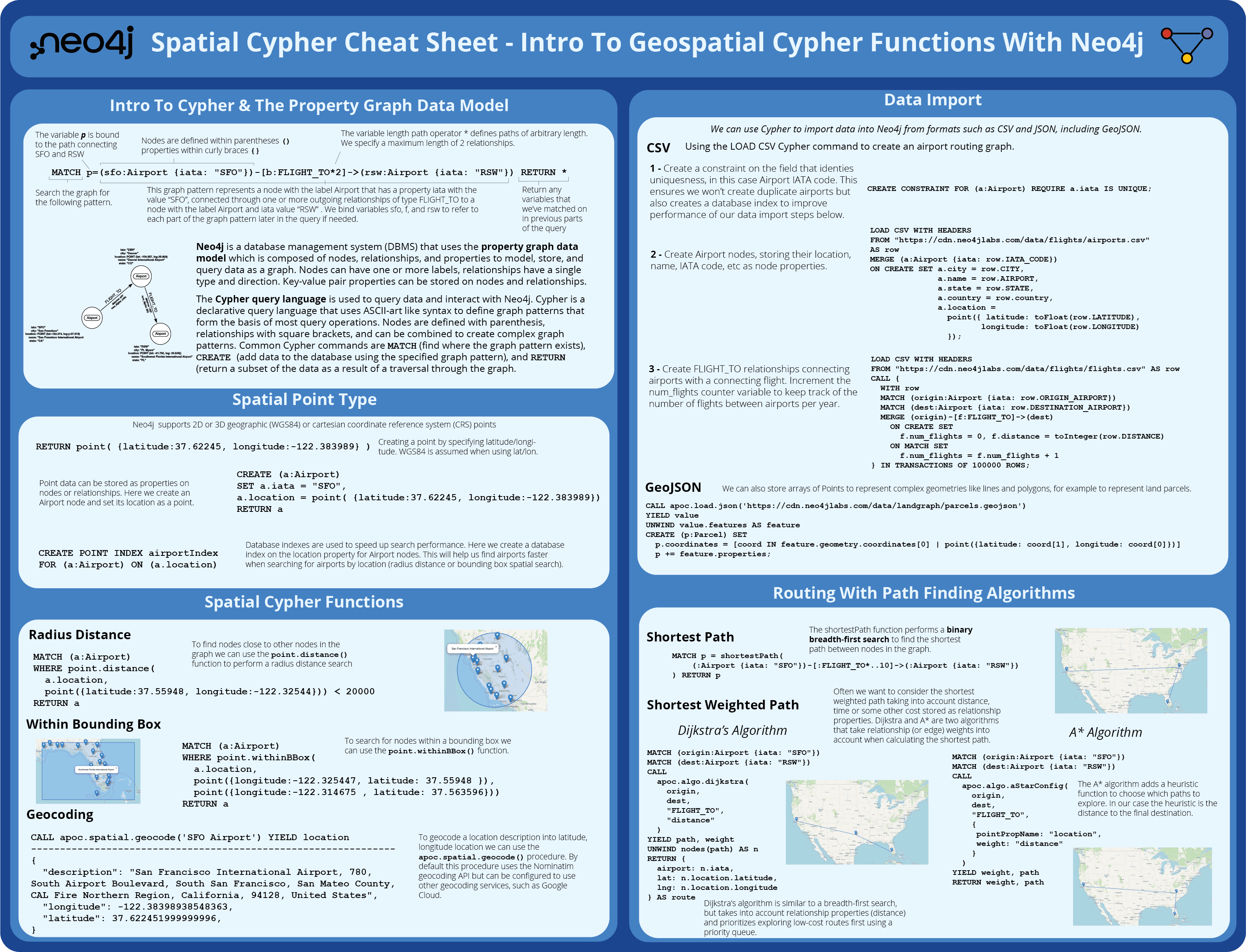
The first page of the Spatial Cypher Cheat Sheet introduces Cypher and the property graph data model, the spatial types available in the Neo4j database, as well as some of the spatial functions availabe in Cypher. We also touch on importing geospatial data into Neo4j (from CSV and GeoJSON) as well as some of the path-finding algorithms (breadth-first search, Dijkstra’s Algorithm, and A*).

Page 2 of the Spatial Cypher Cheat Sheet covers using Neo4j with Python. First, using the Neo4j Python driver to query data from Neo4j to build a GeoDataFrame. We then explore using the OSMNx Python package for fetching data from OpenStreetMap to load a road network into Neo4j.

You can download the PDF version of the Spatial Cypher Cheat Sheet, or read on for the same content in the rest of this blog post.

Introduction To Geospatial Cypher Functions With Neo4j

• Intro To Cypher & The Property Graph Data Model
• Spatial Point Type
• Spatial Cypher Functions
• Data Import
• Routing With Path Finding Algorithms

Using Neo4j With Python

• The Neo4j Python Driver
• Creating A GeoDataFrame From Data Stored In Neo4j
• Working With OpenStreetMap Data
• Loading A Road Network With OSMNx
• Analyzing and Visualizing Road Networks With Neo4j Bloom And Graph Data Science

Introduction To Geospatial Cypher Functions With Neo4j#

Intro To Cypher And The Property Graph Data Model#

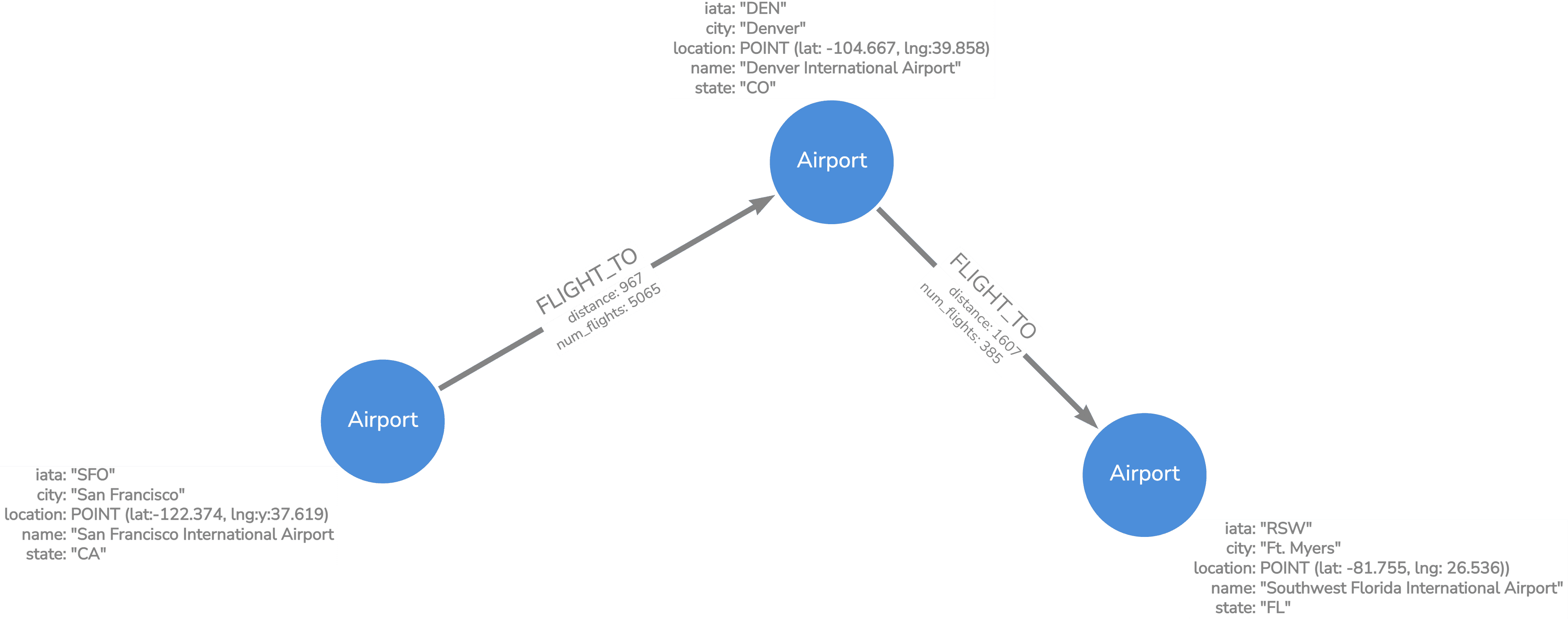
Neo4j is a database management system (DBMS) that uses the property graph data model which is composed of nodes, relationships, and properties to model, store, and query data as a graph. Nodes can have one or more labels, relationships have a single type and direction. Key-value pair properties can be stored on nodes and relationships.

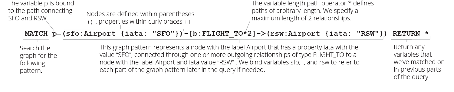
The Cypher query language is used to query data and interact with Neo4j. Cypher is a declarative query language that uses ASCII-art like syntax to define graph patterns that form the basis of most query operations. Nodes are defined with parenthesis, relationships with square brackets, and can be combined to create complex graph patterns. Common Cypher commands are MATCH (find where the graph pattern exists), CREATE (add data to the database using the specified graph pattern), and RETURN (return a subset of the data as a result of a traversal through the graph.

MATCH (sfo:Airport {iata: “SFO”})-[b:FLIGHT_TO*]->(rsw:Airport {iata: “RSW”}) RETURN *

Spatial Point Type#

Neo4j supports 2D or 3D geographic (WGS84) or cartesian coordinate reference system (CRS) points. Here we create a point by specifying latitude/longitude, WGS84 is assumed when using latitude/longitude:

RETURN point( {latitude:37.62245, longitude:-122.383989} )

Point data can be stored as properties on nodes or relationships. Here we create an Airport node and set its location as a point.

CREATE (a:Airport)
SET a.iata = "SFO",
a.location = point( {latitude:37.62245, longitude:-122.383989})
RETURN a

Database indexes are used to speed up search performance. Here we create a database index on the location property for Airport nodes. This will help us find airports faster when searching for airports by location (radius distance or bounding box spatial search).

CREATE POINT INDEX airportIndex FOR (a:Airport) ON (a.location)

Spatial Cypher Functions#

Radius Distance Search

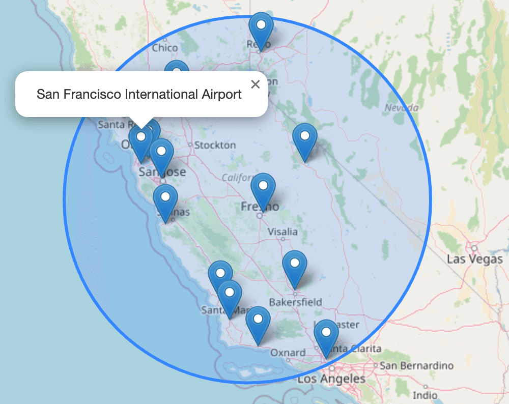
To find nodes close to a point or other nodes in the graph we can use the point.distance() function to perform a radius distance search

MATCH (a:Airport)
WHERE point.distance(
  a.location,
  point({latitude:37.55948, longitude:-122.32544})) < 20000
RETURN a

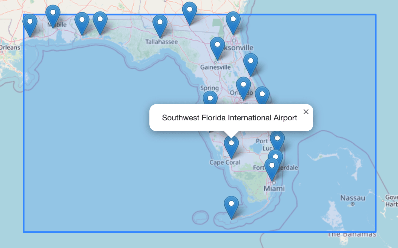
Within Bounding Box

To search for nodes within a bounding box we can use the point.withinBBox() function.

MATCH (a:Airport)
WHERE point.withinBBox(
  a.location,
  point({longitude:-122.325447, latitude: 37.55948 }),
  point({longitude:-122.314675 , latitude: 37.563596}))
RETURN a

See also my other blog post that goes into a bit more detail on spatial search functionality with Neo4j, including point in polygon: Spatial Search Functionality With Neo4j

Geocoding

To geocode a location description into latitude, longitude location we can use the apoc.spatial.geocode() procedure. By default this procedure uses the Nominatim geocoding API but can be configured to use other geocoding services, such as Google Cloud.

CALL apoc.spatial.geocode('SFO Airport') YIELD location
---------------------------------------------------------------
{
  "description": "San Francisco International Airport, 780, South Airport Boulevard, South San Francisco, San Mateo County, CAL Fire Northern Region, California, 94128, United States",
  "longitude": -122.38398938548363,
  "latitude": 37.622451999999996,
}

Data Import#

We can use Cypher to import data into Neo4j from formats such as CSV and JSON, including GeoJSON.

CSV

Using the LOAD CSV Cypher command to create an airport routing graph.

1 - Create a constraint on the field that identies uniquesness, in this case Airport IATA code. This ensures we won’t create duplicate airports but also creates a database index to improve performance of our data import steps below.

CREATE CONSTRAINT FOR (a:Airport) REQUIRE a.iata IS UNIQUE;

2 - Create Airport nodes, storing their location, name, IATA code, etc as node properties.

LOAD CSV WITH HEADERS
FROM "https://cdn.neo4jlabs.com/data/flights/airports.csv"
AS row
MERGE (a:Airport {iata: row.IATA_CODE})
ON CREATE SET a.city = row.CITY,
              a.name = row.AIRPORT,
              a.state = row.STATE,
              a.country = row.country,
              a.location =
                point({ latitude: toFloat(row.LATITUDE),
                       longitude: toFloat(row.LONGITUDE)
                });

3 - Create FLIGHT_TO relationships connecting airports with a connecting flight. Increment the num_flights counter variable to keep track of the number of flights between airports per year.

LOAD CSV WITH HEADERS
FROM "https://cdn.neo4jlabs.com/data/flights/flights.csv" AS row
CALL {
  WITH row
  MATCH (origin:Airport {iata: row.ORIGIN_AIRPORT})
  MATCH (dest:Airport {iata: row.DESTINATION_AIRPORT})
  MERGE (origin)-[f:FLIGHT_TO]->(dest)
    ON CREATE SET
      f.num_flights = 0, f.distance = toInteger(row.DISTANCE)
    ON MATCH SET
      f.num_flights = f.num_flights + 1
} IN TRANSACTIONS OF 100000 ROWS;

GeoJSON

We can also store arrays of Points to represent complex geometries like lines and polygons, for example to represent land parcels.

CALL apoc.load.json('https://cdn.neo4jlabs.com/data/landgraph/parcels.geojson')
YIELD value
UNWIND value.features AS feature
CREATE (p:Parcel) SET
  p.coordinates = [coord IN feature.geometry.coordinates[0] | point({latitude: coord[1], longitude: coord[0]})]
  p += feature.properties;

Routing With Path Finding Algorithms#

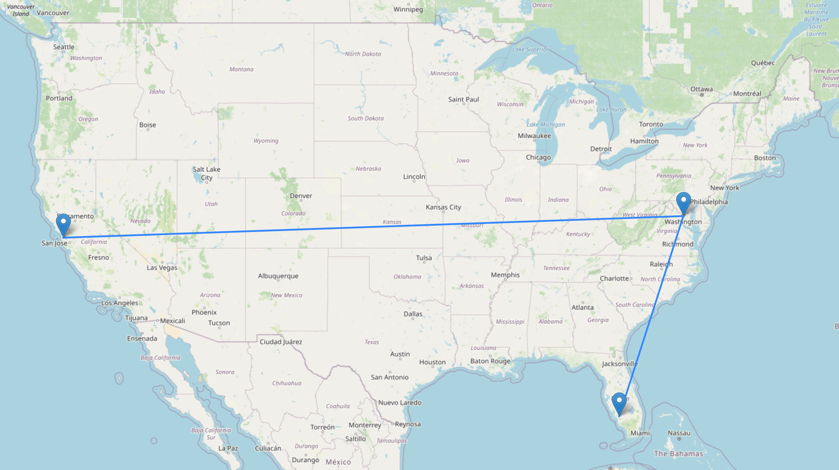
Shortest Path

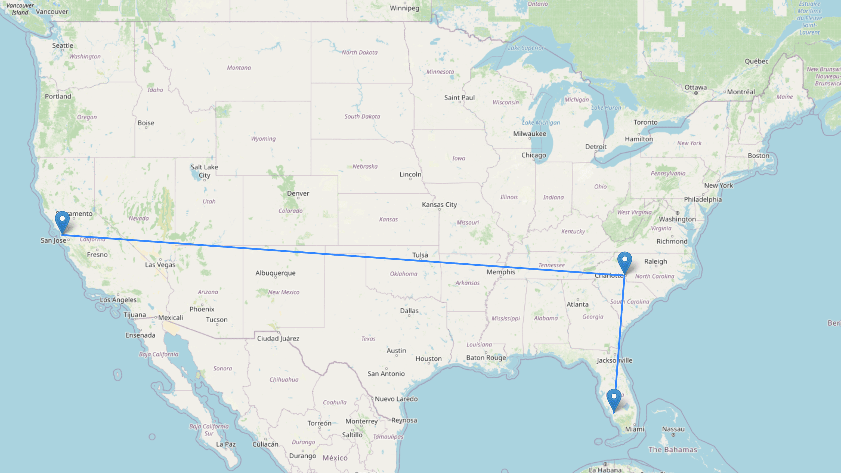
The shortestPath function performs a binary breadth-first search to find the shortest path between nodes in the graph.

MATCH p = shortestPath(
    (:Airport {iata: "SFO"})-[:FLIGHT_TO*..10]->(:Airport {iata: "RSW"})
) RETURN p

Shortest Weighted Path

Often we want to consider the shortest weighted path taking into account distance, time or some other cost stored as relationship properties. Dijkstra and A* are two algorithms that take relationship (or edge) weights into account when calculating the shortest path.

Dijkstra's Algorithm

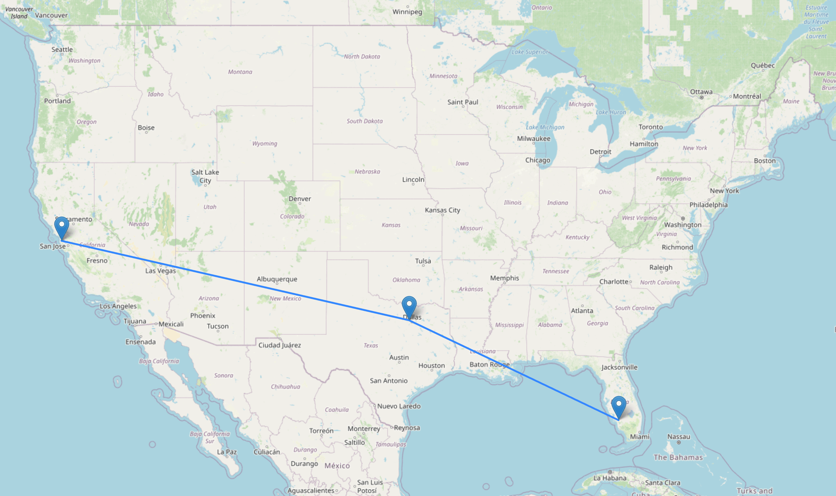
Dijkstra’s algorithm is similar to a breadth-first search, but takes into account relationship properties (distance) and prioritizes exploring low-cost routes first using a priority queue.

MATCH (origin:Airport {iata: "SFO"})
MATCH (dest:Airport {iata: "RSW"})
CALL
  apoc.algo.dijkstra(
    origin,
    dest,
    "FLIGHT_TO",
    "distance"
  )
YIELD path, weight
UNWIND nodes(path) AS n
RETURN {
  airport: n.iata,
  lat: n.location.latitude,
  lng: n.location.longitude
} AS route

A* Algorithm

The A* algorithm adds a heuristic function to choose which paths to explore. In our case the heuristic is the distance to the final destination.

MATCH (origin:Airport {iata: "SFO"})
MATCH (dest:Airport {iata: "RSW"})
CALL
  apoc.algo.aStarConfig(
    origin,
    dest,
    "FLIGHT_TO",
    {
     pointPropName: "location",
     weight: "distance"
    }
  )
YIELD weight, path
RETURN weight, path

There are additional path-finding algorithms available in Neo4j's Graph Data Science Library.

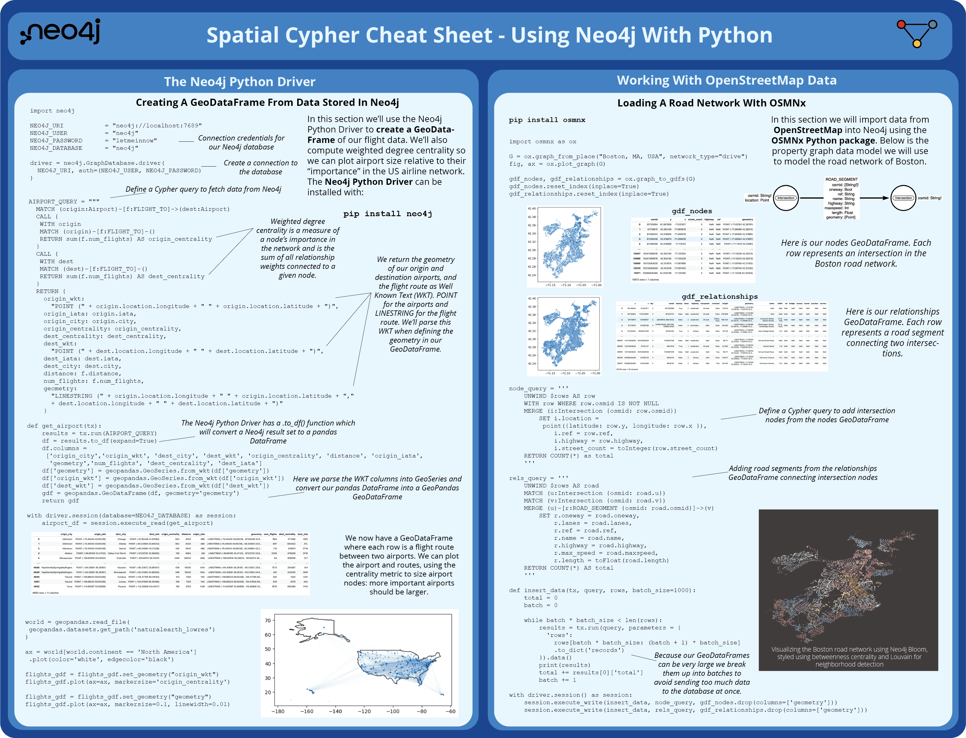
Using Neo4j With Python For Geospatial Data#

The Neo4j Python Driver#

In this section we’ll use the Neo4j Python Driver to create a GeoDataFrame of our flight data. We’ll also compute weighted degree centrality so we can plot airport size relative to their “importance” in the US airline network. The Neo4j Python Driver can be installed with:

pip install neo4j

Creating A GeoDataFrame From Data Stored In Neo4j

First we import the neo4j Python package, define our connection credentials for our Neo4j instance (here we are using a local Neo4j instance), and create a driver instance.

import neo4j

NEO4J_URI           = "neo4j://localhost:7689"
NEO4J_USER          = "neo4j"
NEO4J_PASSWORD      = "letmeinnow"
NEO4J_DATABASE      = "neo4j"

driver = neo4j.GraphDatabase.driver(
  NEO4J_URI, auth=(NEO4J_USER, NEO4J_PASSWORD)
)

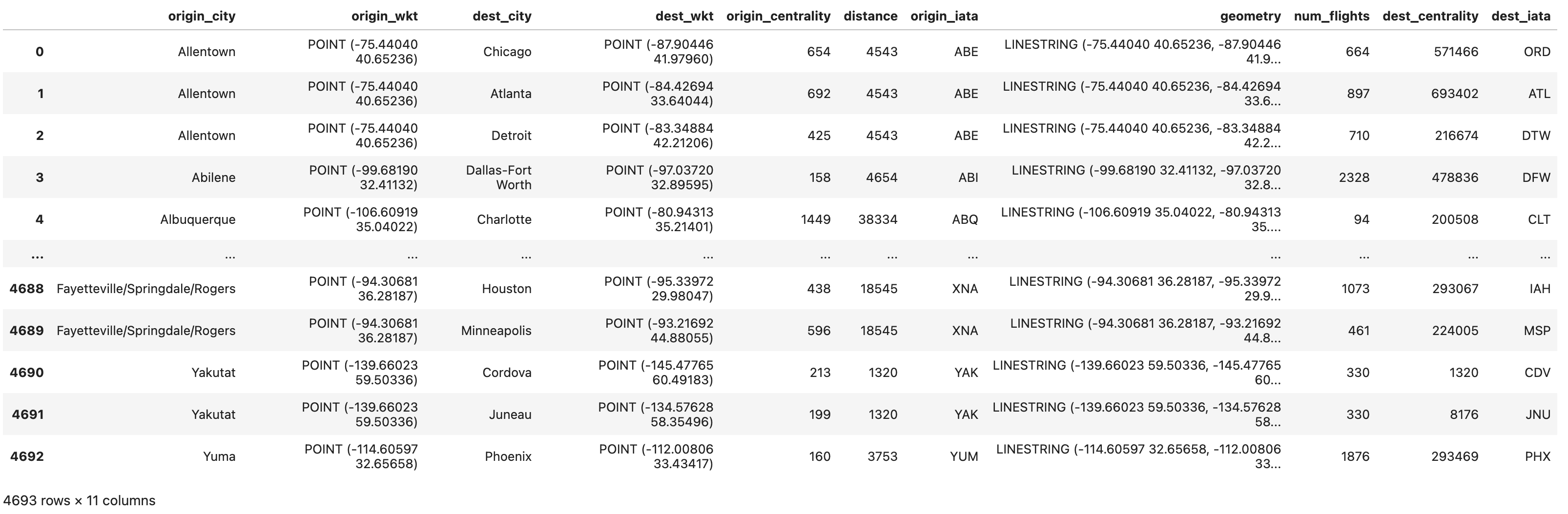
Next, we define a Cypher query to fetch data from Neo4j. In addition to fetching each flight between airports we compute weighted degree centrality, a measure of each node's importance in the network, the sum of all relationship weights connected to a given node, in this case the number of flights per year for each airport.

We also return the geometry of our origin and destination airports, and the flight route as Well Known Text (WKT). POINT for the airports and LINESTRING for the flight route. We’ll parse this WKT when defining the geometry in our GeoDataFrame.

AIRPORT_QUERY = """
  MATCH (origin:Airport)-[f:FLIGHT_TO]->(dest:Airport)
  CALL {
   WITH origin
   MATCH (origin)-[f:FLIGHT_TO]-()
   RETURN sum(f.num_flights) AS origin_centrality
  }
  CALL {
   WITH dest
   MATCH (dest)-[f:FLIGHT_TO]-()
   RETURN sum(f.num_flights) AS dest_centrality
  }
  RETURN {
    origin_wkt:
      "POINT (" + origin.location.longitude + " " + origin.location.latitude + ")",
    origin_iata: origin.iata,
    origin_city: origin.city,
    origin_centrality: origin_centrality,
    dest_centrality: dest_centrality,
    dest_wkt:
      "POINT (" + dest.location.longitude + " " + dest.location.latitude + ")",
    dest_iata: dest.iata,
    dest_city: dest.city,
    distance: f.distance,
    num_flights: f.num_flights,
    geometry:
      "LINESTRING (" + origin.location.longitude + " " + origin.location.latitude + ","
      + dest.location.longitude + " " + dest.location.latitude + ")"
    }
    """

Next we define a Python function to execute our Cypher query and process the results into a GeoPandas GeoDataFrame. The Neo4j Python driver has a .to_df() method which will convert a Neo4j result set to a Pandas DataFrame. Note that we parse the WKT columns into GeoSeries and convert the pandas DataFrame into a GeoPandas GeoDataFrame.

def get_airport(tx):
    results = tx.run(AIRPORT_QUERY)
    df = results.to_df(expand=True)
    df.columns =
     ['origin_city','origin_wkt', 'dest_city', 'dest_wkt', 'origin_centrality', 'distance', 'origin_iata',
      'geometry','num_flights', 'dest_centrality', 'dest_iata']
    df['geometry'] = geopandas.GeoSeries.from_wkt(df['geometry'])
    df['origin_wkt'] = geopandas.GeoSeries.from_wkt(df['origin_wkt'])
    df['dest_wkt'] = geopandas.GeoSeries.from_wkt(df['dest_wkt'])
    gdf = geopandas.GeoDataFrame(df, geometry='geometry')
    return gdf

with driver.session(database=NEO4J_DATABASE) as session:
    airport_df = session.execute_read(get_airport)

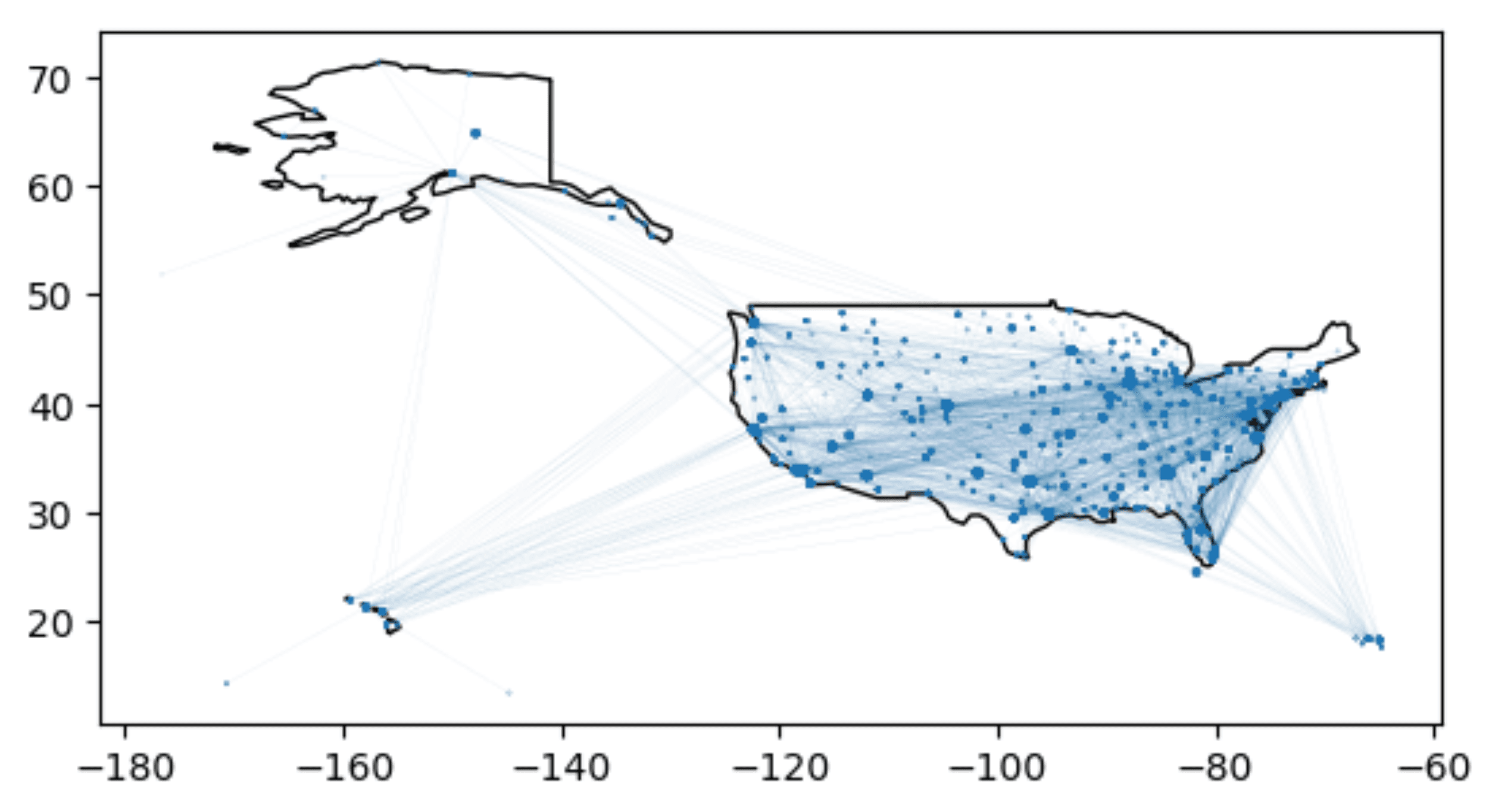
We now have a GeoDataFrame where each row is a flight route between two airports. We can plot the airport and routes, using the centrality metric to size airport nodes: more important airports should be larger.

world = geopandas.read_file(
 geopandas.datasets.get_path('naturalearth_lowres')
)

ax = world[world.continent == 'North America']
 .plot(color='white', edgecolor='black')

flights_gdf = flights_gdf.set_geometry("origin_wkt")
flights_gdf.plot(ax=ax, markersize='origin_centrality')

flights_gdf = flights_gdf.set_geometry("geometry")
flights_gdf.plot(ax=ax, markersize=0.1, linewidth=0.01)

Working With OpenStreetMap Data#

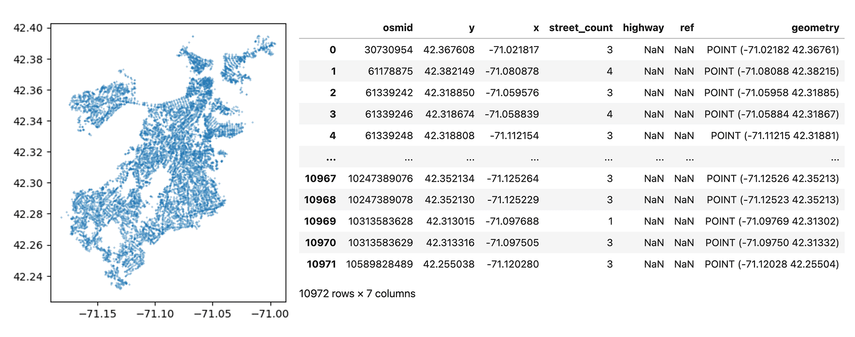
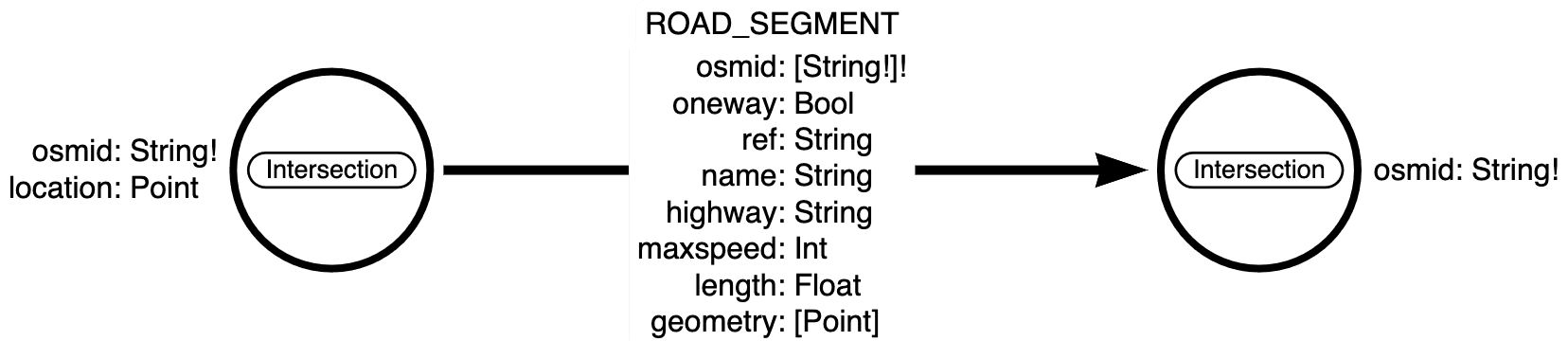
In this section we will import data from OpenStreetMap into Neo4j using the OSMNx Python package. Below is the property graph data model we will use to model the road network of Boston.

pip install osmnx

Loading A Road Network With OSMNx#

import osmnx as ox

G = ox.graph_from_place("Boston, MA, USA", network_type="drive")
fig, ax = ox.plot_graph(G)

gdf_nodes, gdf_relationships = ox.graph_to_gdfs(G)
gdf_nodes.reset_index(inplace=True)
gdf_relationships.reset_index(inplace=True)

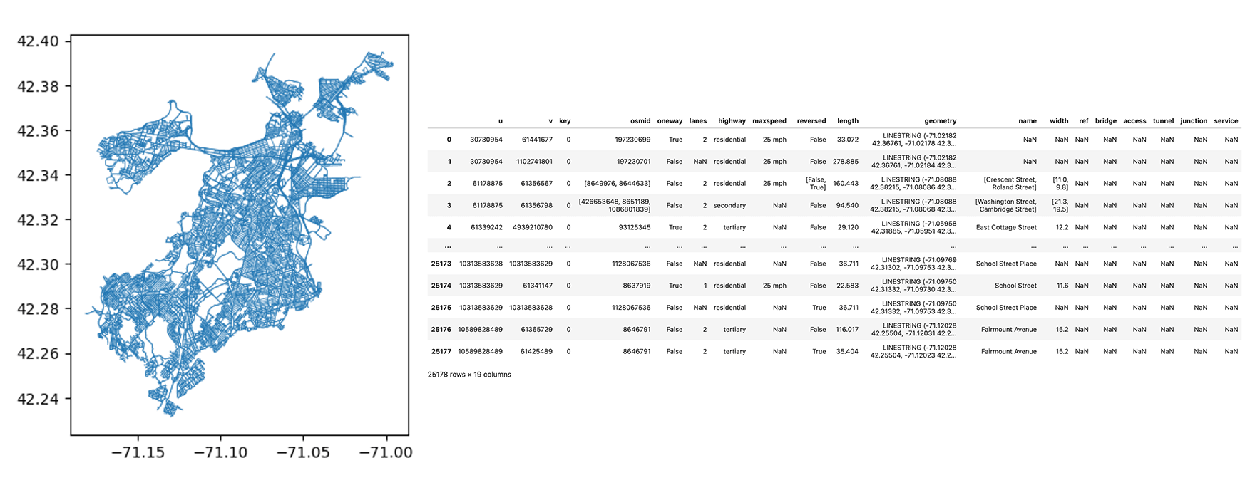
Here is our nodes GeoDataFrame. Each row represents an intersection in the Boston road network.:

Here is our relationships GeoDataFrame. Each row represents a road segment connecting two intersections.

Define a Cypher query to add intersection nodes from the nodes GeoDataFrame

Adding road segments from the relationships GeoDataFrame connecting intersection nodes

Because our GeoDataFrames can be very large we break them up into batches to avoid sending too much data to the database at once.

node_query = '''
    UNWIND $rows AS row
    WITH row WHERE row.osmid IS NOT NULL
    MERGE (i:Intersection {osmid: row.osmid})
        SET i.location =
         point({latitude: row.y, longitude: row.x }),
            i.ref = row.ref,
            i.highway = row.highway,
            i.street_count = toInteger(row.street_count)
    RETURN COUNT(*) as total
    '''

rels_query = '''
    UNWIND $rows AS road
    MATCH (u:Intersection {osmid: road.u})
    MATCH (v:Intersection {osmid: road.v})
    MERGE (u)-[r:ROAD_SEGMENT {osmid: road.osmid}]->(v)
        SET r.oneway = road.oneway,
            r.lanes = road.lanes,
            r.ref = road.ref,
            r.name = road.name,
            r.highway = road.highway,
            r.max_speed = road.maxspeed,
            r.length = toFloat(road.length)
    RETURN COUNT(*) AS total
    '''

def insert_data(tx, query, rows, batch_size=1000):
    total = 0
    batch = 0

    while batch * batch_size < len(rows):
        results = tx.run(query, parameters = {
          'rows':
            rows[batch * batch_size: (batch + 1) * batch_size]
            .to_dict('records')
        }).data()
        print(results)
        total += results[0]['total']
        batch += 1

with driver.session() as session:
    session.execute_write(insert_data, node_query, gdf_nodes.drop(columns=['geometry']))
    session.execute_write(insert_data, rels_query, gdf_relationships.drop(columns=['geometry']))

Analyzing and Visualizing Road Networks With Neo4j Bloom and Graph Data Science#

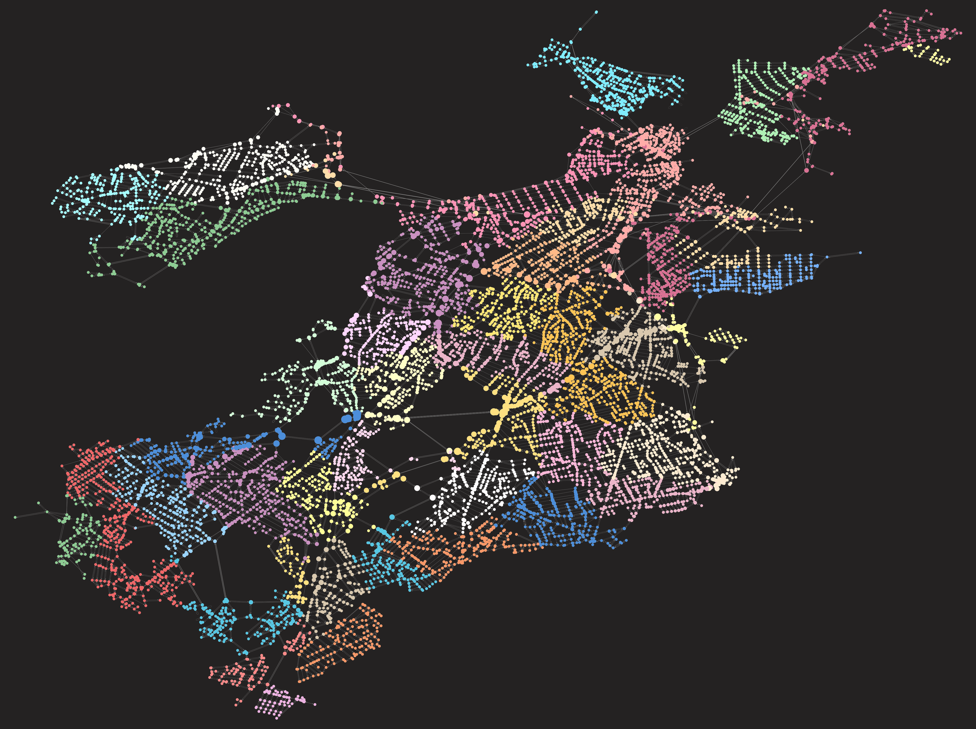
Visualizing the Boston road network using Neo4j Bloom, styled using betweenness centrality and Louvain for neighborhood detection

In this post we introduced some of the spatial functionality natively supported by Neo4j including the point type and related Cypher functions and demonstrated how to accomplish various spatial search operations as well as a brief look at routing with graph algorithms.

Resources#

• Cypher manual for spatial Cypher functions
• Spatial search map example code
• Daylight Earth Table
• Importing Daylight Earth Table points of interest into Neo4j (Python code)
• Spatial search Leaflet.js + Neo4j demo code